Wallabies will prove you wrong

About data structures and other things as well

Did you know that female wallabies (and some other marsupials) have two uteri? Talk about power 💪! And if that weren’t cool enough, they’re basically pregnant their entire lives. When the first walla-baby developing in one uterus is big enough, the mother conceives again. The new embryo stays in developmental arrest until the first young is born, grows, and eventually leaves her pouch. Then, once that embryo starts to develop further, she gets pregnant again — and so the cycle continues…

If you also think it’s pretty impressive, you can check it out here.

Photo by Ethan Brooke, source

And why am I telling you all this? Well, I’m a zoologist, and I think it’s cool! Besides, today I wanted to talk about the structure of objects — a topic I found pretty boring as a student. And, okay, maybe it’s still a bit dull, but that doesn’t mean it’s unimportant. I dare to say that 5% of the errors that make R throw you a red error message (and maybe burst a few eye capillaries) are due to issues with object structure. 50% of errors are, of course, typos and missing commas.

You can get the data here — let’s stick to blue tits as I don’t have much data on wallabies.

### Loading the data ###

library(readr)

blue_tits <- read_csv("../data/blue_tits.csv") # Remember to use the correct file pathway

Then let’s check the structure of our data:

str(blue_tits)

What is the output?

The first column, “Nestbox”, contains characters (also known as strings or character strings), whereas the other two columns, “Laying_day” and “Hatching_day” contain numerical values. You can also see that the last two columns have been described as contacting “doubles” (<dbl>). We won’t worry about it too much, as it is just a way R and some other languages classify numbers with or without decimal places.

Okay, that makes sense, right?

But what would happen if we wanted to add a new row of data to our existing data frame, using rbind() function, and accidentally denoted missing data as “Na” (instead of typing “NA” that is recognised by R as a missing value)?

blue_tits_updated <- rbind(blue_tits, data.frame(Nestbox = "A333", 
                                                 Laying_day = 4, 
                                                 Hatching_day = "Na"))
str(blue_tits_updated)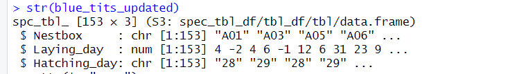

You can see how this small mistake caused the entire column to be categorized as containing character values.

But why are we checking all of that? Is it really that bad?

To answer this question, try typing this into the console (remembering about removing NAs!):

mean(blue_tits_updated$Hatching_day, na.rm = TRUE)

We are trying to get the average value of when birds in our population hatch, but instead, R probably shared with you a nice error message:

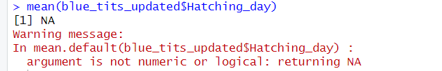
Computers aren’t particularly creative. If you type “2 + 2” in the console, R will give you 4. But if you type “two + two”, it gets lost. That’s because R is programmed to perform calculations on numbers, not on characters. In this case, R won’t return a mean if it doesn’t recognize the data as numerical.

That’s why it is so important that you and R are interpreting your data in the same way. You need to guide R to understand your intentions. To do so, type:

blue_tits_updated$Hatching_day <- as.numeric(blue_tits_updated$Hatching_day)

After executing this command, you probably got the “NAs introduced by coercion” message, which means that R treated the character values as missing values and replaced them with NAs.

You can check whether we are right, by executing the tail() command, which displays the last rows of a data frame:

tail(blue_tits_updated)

Now you should be able to run the mean() command and get 33.3 as an output.

Making sure that R properly recognises the data structure can be also important in other cases.

Let’s imagine we want to compare two groups of birds. For this exercise, we’ll assign each nest box to one of two groups, A or Z, semi-randomly (since the nest boxes are listed alphabetically).

A and Z will be our factors — labels that categorise values.

vector <- c(rep("A",76), rep("Z",77)) #we have 153 nestboxes in our df, hence 76 + 77

blue_tits_updated$Group <- vector

The rep() function (short for “replicate”) creates 76 "A" and 77 "Z" values. This way I don’t have to type them manually — I'm lazy, and that would take up a lot of space! The c() function (short for “concatenate”) then glues all these values into one vector ( a collection of values).

Now we can easily calculate the average hatching day of these two groups by typing:

tapply(blue_tits_updated$Hatching_day, blue_tits_updated$Group, mean, na.rm = TRUE)

You can access the documentation for the tapply() function here, but we are using it to simply apply the mean() function on the “Hatching_day” column based on the “Group” factor. We also exclude the NAs values from our calculations — they are a pain and you can read more about it here.

Usually, R recognizes that “As” and “Zs” represent grouping factors, but sometimes it may treat them as simple character values and refuse to cooperate. In such cases, we can help R understand our intentions by explicitly converting the “Group” column into a factor column:

blue_tits_updated$Group <- as.factor(blue_tits_updated$Group)

That should solve the problem!

That’s all for today, chat with you next week,

Aga

PS: Here is the survey in which you can tell me what R topic you find particularly confusing and why you want to learn it so that we can shape this space together!